DreaMS Atlas

The DreaMS Atlas is a large-scale molecular network containing 201 million MS/MS spectra from the MassIVE GNPS repository, constructed using DreaMS embeddings. Each node in the network corresponds to a mass spectrum derived from a specific biological or environmental sample (e.g., human skin or blood, plant extracts, marine environments, food, and many others). Each edge represents a DreaMS similarity, linking a node to its three nearest neighbors across the entire MassIVE GNPS. This tutorial demonstrates various methods for exploring and analyzing the DreaMS Atlas through a user-friendly API.

Initialization

Import all the necessary packages

import networkx as nx
from rdkit import Chem
import numpy as np
import seaborn as sns
import matplotlib.pyplot as plt
import dreams.utils.plots as plots
import dreams.utils.spectra as su
from dreams.api import DreaMSAtlas
from dreams.utils.misc import networkx_to_dataframe
from dreams.definitions import *
%reload_ext autoreload
%autoreload 2

Initialize the DreaMS Atlas. Please note that the first initialization involves downloading over 400 GB of data files. However, once the files are downloaded, they accessed directly from the disk, so there’s no need to load all the data into memory, eliminating the requirement for a RAM-intensive machine to work with the Atlas.

ℹ️ In future updates, we plan to develop a web server that will allow access to the DreaMS Atlas from a remote server, removing the need to host all the data locally. Future release will also include the ability to extend the Atlas with new nodes and to query the Atlas using a spectrum of interest by DreaMS similarity.

atlas = DreaMSAtlas()

Initializing DreaMS Atlas data structures...
Loaded spectral library (79,300 spectra).
Loaded GeMS-C1 dataset (75,520,646 spectra).
Loaded DreaMS Atlas edges (134,524,452 edges).
Loaded DreaMS Atlas nodes representing DreaMS k-NN clusters of GeMS-C1 (33,631,113 nodes).
Loaded LSH clusters of DreaMS Atlas nodes representing GeMS-C (201,223,336 spectra).

Accesing data from the Atlas

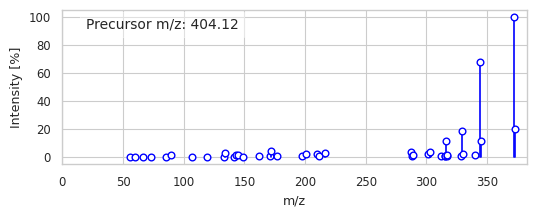
Let’s pick one of the 76 million spectra in GeMS-C1 dataset.

i = 37552437
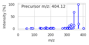
atlas.get_data(i, plot=True, return_spec=False, msv_metadata=True)

{37552437: {'DreaMS_embedding': array([-0.8768827 , -0.41617227,  0.02967745, ..., -1.2626797 ,
          1.6408856 , -0.64122283], dtype=float32),
  'RT': 550.4616,
  'charge': 1,
  'instrument accuracy est.': 0.00013683233,
  'lsh': -450688754114588762,
  'name': '20160906_pgk965_SloanSurfaceProject_Metabolomics_2-21',
  'precursor_mz': 404.1232,
  'msv_id': 'MSV000086209',
  'msv_species': 'NCBITaxon:2;NCBITaxon:4751',
  'msv_species_resolved': 'Bacteria (NCBITaxon:2)',
  'msv_instrument': nan,
  'msv_instrument_resolved': nan,
  'msv_title': 'GNPS - Microbial and metabolic succession on common building materials under high humidity conditions',
  'msv_description': 'Despite considerable efforts to characterize the microbial ecology of the built environment, the metabolic mechanisms underpinning microbial colonization and successional dynamics remain unclear, particularly at high moisture conditions. Here, we applied bacterial/viral particle counting, qPCR, amplicon sequencing of the genes encoding 16S and ITS rRNA, and metabolomics to longitudinally characterize the ecological dynamics of four common building materials maintained at high humidity. We varied the natural inoculum provided to each material and wet half of the samples to simulate a potable water leak. Wetted materials had higher growth rates and lower alpha diversity compared to non-wetted materials, and wetting described the majority of the variance in bacterial, fungal, and metabolite structure. Inoculation location was weakly associated with bacterial and fungal beta diversity. Material type influenced bacterial and viral particle abundance and bacterial and metabolic (but not fungal) diversity. Metabolites indicative of microbial activity were identified, and they too differed by material.',
  'msv_create_time': '2020-09-29 08:10:16.0',
  'msv_user': nan,
  'msv_keywords': nan}}

The displayed spectrum represents a single node in the Atlas. In addition to mass spectrometry attributes such as MS/MS peaks, precursor m/z, and retention time, the spectrum is associated with a DreaMS embedding and MassIVE GNPS metadata, which includes, for example, the species studied or the study description.

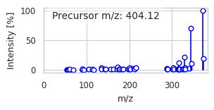
According to the construction of the DreaMS Atlas, each node represents a cluster of MS/MS spectra obtained using DreaMS and LSH. Let us explore the cluster corresponding to the selected node.

dreams_cluster = atlas.get_node_cluster(i, lsh=True)
print(f'Node {i} represents a cluster of {len(dreams_cluster)} spectra with high DreaMS similarity.')
for spec_i, lsh_cluster in dreams_cluster.items():
    print(f'Spectrum with index {spec_i} further represents an LSH cluster of {len(lsh_cluster)} spectra.')
    print('Showing first spectrum:')
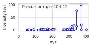
    su.plot_spectrum(lsh_cluster[0][SPECTRUM], prec_mz=lsh_cluster[0][PRECURSOR_MZ], figsize=(3, 1.2))

Node 37552437 represents a cluster of 6 spectra with high DreaMS similarity.
Spectrum with index 32730250 further represents an LSH cluster of 1 spectra.
Showing first spectrum:

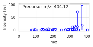
Spectrum with index 32730265 further represents an LSH cluster of 2 spectra.
Showing first spectrum:

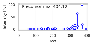
Spectrum with index 32730269 further represents an LSH cluster of 42 spectra.
Showing first spectrum:

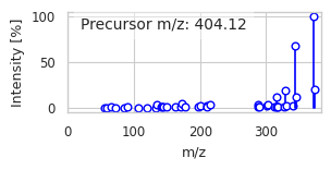
Spectrum with index 37552435 further represents an LSH cluster of 3 spectra.
Showing first spectrum:

Spectrum with index 37552437 further represents an LSH cluster of 5 spectra.
Showing first spectrum:

Spectrum with index 37552438 further represents an LSH cluster of 2 spectra.
Showing first spectrum:

Exploring local structure of the Atlas

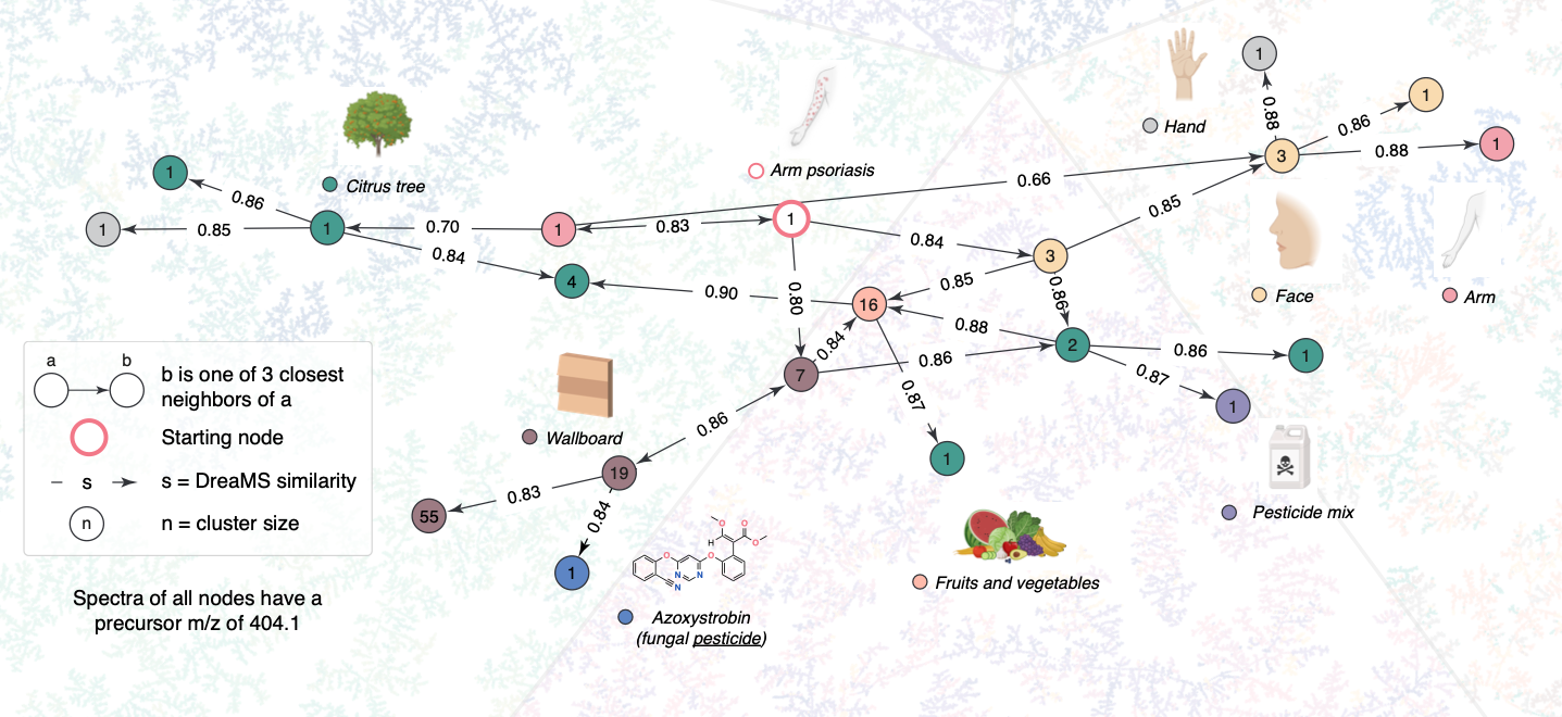
The DreaMS Atlas API allows for the visualization of a neighborhood of a given node as an interactive graph.

i = 37542683
g_nbhd = atlas.get_neighbors(i, n_hops=3, msv_metadata=True)

plots.plot_nx_graph(
    g_nbhd,
    node_attrs=[PRECURSOR_MZ, NAME, SMILES, 'msv_id'],
    node_color_attr='msv_id',
    special_node=i,
    special_nodes=[n[0] for n in g_nbhd.nodes(data=True) if SMILES in n[1]],
    node_size=12
)

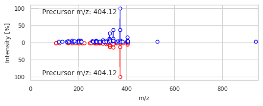
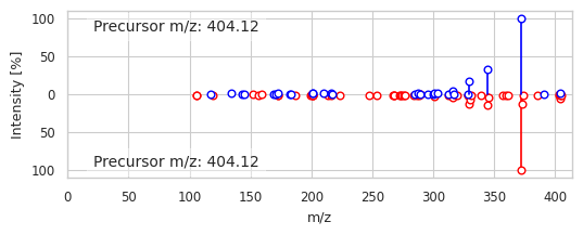
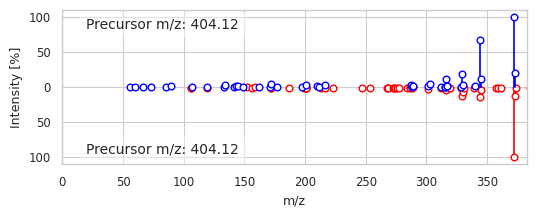
Let’s examine the similarities between three spectra from the neighborhood and our query spectrum of interest. Note that one of the nodes represents an entry from the MoNA spectral library and is therefore annotated with a molecular structure.

for n in list(g_nbhd.nodes(data=True))[-3:]:
    print('Node', n[0])
    su.plot_spectrum(spec=n[1][SPECTRUM], mirror_spec=g_nbhd.nodes[i][SPECTRUM], prec_mz=n[1][PRECURSOR_MZ], mirror_prec_mz=g_nbhd.nodes[i][PRECURSOR_MZ])
    if SMILES in n[1]:
        display(Chem.MolFromSmiles(n[1][SMILES]))

Node 37496414

Node 34207

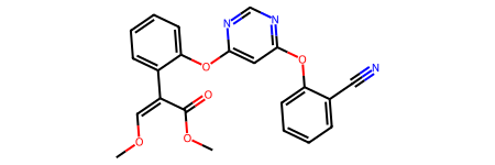
Node 37552437

One can also explore the neighborhood as a pandas data frame.

networkx_to_dataframe(g_nbhd).head()

	node_id	RT	msv_keywords	msv_instrument_resolved	msv_create_time	name	msv_species_resolved	id	DreaMS_embedding	msv_instrument	...	msv_species	charge	lsh	msv_description	spectrum	instrument accuracy est.	msv_id	msv_title	neighbors	edge_weight
0	37542683	309.739990	Skin	maXis	2018-07-31 14:41:27.0	BD4_V14_S2-015_arm_psoriasis_BD4_01_14378	Homo sapiens	None	[-0.10430071, 0.32463387, 1.2688519, 1.7766136...	MS:1001541	...	NCBITaxon:9606	0	-4.529384e+17	GNPS - Skin psoriasis molecular cartography st...	[[106.06563568115234, 106.07821655273438, 119....	0.000712	MSV000082674	GNPS - Skin psoriasis molecular cartography st...	[37542661, 37542656, 37648590]	[0.8408746152701184, 0.829488577059148, 0.7978...
1	37542661	306.300995	Facial cleanser, skin, temporal	maXis	2018-06-01 15:00:35.0	5A9_%20V1_%20Nose_%20D14H0_%20W7_BA9_01_11583	Homo sapiens	None	[0.19762689, 0.17532083, 1.2078881, 1.549347, ...	MS:1001541	...	NCBITaxon:9606	0	-4.529386e+17	MS/MS spectra were collected from face of 6 in...	[[121.03773498535156, 151.0904998779297, 156.0...	0.000614	MSV000082432	GNPS - Colgate facial cleanser longitudinal st...	[37542653, 32640049, 37542632]	[0.8550434399274379, 0.8537323876318667, 0.851...
2	37542656	309.917999	Skin	maXis	2018-07-31 14:41:27.0	BD3_V14_S2-014_arm_healthy_BD3_01_14337	Homo sapiens	None	[0.38015515, -0.5561968, 1.060871, 0.93926096,...	MS:1001541	...	NCBITaxon:9606	0	-4.529386e+17	GNPS - Skin psoriasis molecular cartography st...	[[119.0505599975586, 134.0594482421875, 145.02...	0.000678	MSV000082674	GNPS - Skin psoriasis molecular cartography st...	[37542683, 37542627, 37542661]	[0.829488577059148, 0.7041841665583883, 0.6607...
3	37648590	541.183533	NaN	NaN	2020-09-29 08:10:16.0	20160906_pgk965_SloanSurfaceProject_Metabolomi...	Bacteria (NCBITaxon:2)	None	[-0.18013018, 0.5833932, 1.3610793, 2.4781635,...	NaN	...	NCBITaxon:2;NCBITaxon:4751	1	-4.326744e+17	Despite considerable efforts to characterize t...	[[89.41886901855469, 89.42453002929688, 96.847...	0.000139	MSV000086209	GNPS - Microbial and metabolic succession on c...	[32730262, 37542653, 32640049]	[0.8631632498896021, 0.8612309271933151, 0.842...
4	37542653	349.489990	citrus	maXis 4G	2020-05-15 11:47:12.0	Plate_2_1_820_RE7_01_41664	Citrus sinensis (NCBITaxon:2711)	None	[0.024766939, -0.28584233, 1.1211307, 1.363762...	MS:1002279	...	NCBITaxon:2711	0	-4.529386e+17	Leaf tissues of orange trees extracted with et...	[[130.02940368652344, 133.05169677734375, 134....	0.000519	MSV000085416	GNPS_UCR_citrus_survivor_study_orchard_samples...	[32640049, 37496366, 37542658]	[0.8816033077004346, 0.8651546656827798, 0.864...

5 rows × 24 columns

Exploring global structure of the Atlas

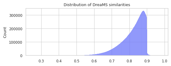
The global structure of the DreaMS Atlas can be analyzed in two ways. First, one can efficiently analyze the graph by accessing its adjacency matrix, which is stored as a sparse array. For example, let’s plot the distribution of the DreaMS similarities representing the graph edges.

A = atlas.csrknn.csr
print('Adjacency matrix shape:', A.shape)
edges = np.asarray(A[A > 0]).ravel()

print('Number of edges:', len(edges))
sns.histplot(edges)
plt.title('Distribution of DreaMS similarities')
plt.show()

Adjacency matrix shape: (33631113, 33631113)
Number of edges: 101104558

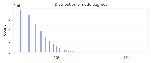
Second, one can work with the Atlas as an igraph graph object, leveraging the many graph analysis methods implemented within the igraph package. For example, let’s plot the distribution of node degrees across the entire Atlas.

G = atlas.csrknn.to_graph()

Retrieving graph edges: 100%|██████████| 33631113/33631113 [03:09<00:00, 177295.81it/s]

degrees = G.degree()
sns.histplot(degrees, log_scale=True, shrink=10)
plt.title('Distribution of node degrees')
plt.show()