Libray matching with DreaMS

Introduction

According to the results presented in our paper, DreaMS embeddings provide a more accurate way to perform library matching than traditional algorithms such as modified cosine similarity or spectral entropy. Library matching is the annotation of a query spectrum with a molecule corresponding to the most similar spectrum in some given spectral library. In this tutorial, we will demonstrate how to perform library matching with DreaMS embeddings using the MassSpecGym dataset as a library, which contains a curated collection of public high-quality MS/MS spectra.

Import necessary libraries.

[1]:

import pandas as pd
import numpy as np
from pathlib import Path
from tqdm import tqdm
from sklearn.metrics.pairwise import cosine_similarity
from rdkit import Chem
import dreams.utils.spectra as su
import dreams.utils.io as io
from dreams.utils.spectra import PeakListModifiedCosine
from dreams.utils.data import MSData
from dreams.api import dreams_embeddings
from dreams.definitions import *

Determination of memory status is not supported on this
 platform, measuring for memoryleaks will never fail

Load data

Load example dataset downloaded from MSV000086206 and MassSpecGym library with pre-computed DreaMS embeddings.

[3]:

in_pth = Path('../data/S_N1.mzML')  # Example dataset
lib_pth = Path('../data/MassSpecGym_DreaMS.hdf5')  # MassSpecGym library

[4]:

msdata_lib = MSData.load(lib_pth)
embs_lib = msdata_lib[DREAMS_EMBEDDING]
print('Shape of the library embeddings:', embs_lib.shape)

Shape of the library embeddings: (231104, 1024)

[6]:

msdata = MSData.load(in_pth)
embs = dreams_embeddings(msdata)
print('Shape of the query embeddings:', embs.shape)

Computing DreaMS embedding: 100%|██████████| 3809/3809 [01:42<00:00, 37.22it/s]

Shape of the query embeddings: (3809, 1024)

Perform library matching

Compute all cosine similarity between the query and library DreaMS embeddings.

[7]:

sims = cosine_similarity(embs, embs_lib)
sims.shape

[7]:

(3809, 231104)

Choose top-k candidates with the highest similarity per query spectrum.

[8]:

k = 5
topk_cands = np.argsort(sims, axis=1)[:, -k:][:, ::-1]
topk_cands.shape

[8]:

(3809, 5)

Organize the results in a DataFrame with the most important library metadata, such as library SMILES.

[15]:

# Construct a DataFrame with the top-k candidates for each spectrum and their corresponding similarities
df = []
cos_sim = su.PeakListModifiedCosine()
for i, topk in enumerate(tqdm(topk_cands)):
    for n, j in enumerate(topk):
        df.append({
            'feature_id': i + 1,
            'precursor_mz': msdata.get_values(PRECURSOR_MZ, i),
            'RT': msdata.get_values(RT, i),
            'topk': n + 1,
            'library_j': j,
            'library_SMILES': msdata_lib.get_smiles(j),
            'library_ID': msdata_lib.get_values('IDENTIFIER', j),
            'library_precursor_mz': msdata_lib.get_values(PRECURSOR_MZ, j),
            'library_adduct': msdata_lib.get_values(ADDUCT, j),
            'library_collision_energy': msdata_lib.get_values('COLLISION_ENERGY', j),
            'DreaMS_similarity': sims[i, j],
            'Modified_cosine_similarity': cos_sim(
                spec1=msdata.get_spectra(i),
                prec_mz1=msdata.get_prec_mzs(i),
                spec2=msdata_lib.get_spectra(j),
                prec_mz2=msdata_lib.get_prec_mzs(j),
            ),
            'i': i,
            'j': j,
        })
df = pd.DataFrame(df)

# Sort hits by DreaMS similarity
df_top1 = df[df['topk'] == 1].sort_values('DreaMS_similarity', ascending=False)
df = df.set_index('feature_id').loc[df_top1['feature_id'].values].reset_index()
df

100%|██████████| 3809/3809 [03:29<00:00, 18.17it/s]

[15]:

	feature_id	precursor_mz	RT	topk	library_j	library_SMILES	library_ID	library_precursor_mz	library_adduct	library_collision_energy	DreaMS_similarity	Modified_cosine_similarity	i	j
0	344	565.235133	185.953374	1	217668	CC(=O)N(CCCC[C@@H](C(=O)O)NC(=O)CC(CC(=O)N[C@@...	MassSpecGymID0396609	565.23000	[M+H]+	NaN	0.979676	0.999883	343	217668
1	344	565.235133	185.953374	2	156591	CC1=C2C(=NC=NN2C=C1NC(=O)OC[C@@H]3COCCN3)NC4=C...	MassSpecGymID0225965	531.22629	[M+H]+	20.0	0.609247	0.643832	343	156591
2	344	565.235133	185.953374	3	161476	CN1C2=C(C=CC(=C2)C3=CC=C(C=C3)C[C@@H](C#N)NC(=...	MassSpecGymID0231755	421.18703	[M+H]+	30.0	0.601104	0.488964	343	161476
3	344	565.235133	185.953374	4	135639	CCC1=CC(=C(S1)NC(=O)CCN2CCOCC2)C(=O)OCC	MassSpecGymID0203635	341.15295	[M+H]+	20.0	0.595223	0.664075	343	135639
4	344	565.235133	185.953374	5	155803	CC(=O)NCCCOC1=CC=C(C=C1)C(=O)N2CCC(CC2)N3C(=O)...	MassSpecGymID0225137	450.23873	[M+H]+	30.0	0.570048	0.725630	343	155803
...	...	...	...	...	...	...	...	...	...	...	...	...	...	...
19040	1789	237.110323	476.531454	1	104889	CC(=CCOC1=C2C=CC(=O)OC2=CC3=C1C=CO3)C	MassSpecGymID0151614	293.08000	[M+Na]+	NaN	0.342242	0.831349	1788	104889
19041	1789	237.110323	476.531454	2	181939	CC1=C(N2C(C(C2=O)[NH3+])SC1)C(=O)[O-]	MassSpecGymID0268406	237.03000	[M+Na]+	NaN	0.328011	0.700030	1788	181939
19042	1789	237.110323	476.531454	3	181941	CC1=C(N2C(C(C2=O)[NH3+])SC1)C(=O)[O-]	MassSpecGymID0268414	237.03000	[M+Na]+	NaN	0.327554	0.809387	1788	181941
19043	1789	237.110323	476.531454	4	104897	CC(=CCOC1=C2C=CC(=O)OC2=CC3=C1C=CO3)C	MassSpecGymID0151624	293.08000	[M+Na]+	NaN	0.327202	0.737573	1788	104897
19044	1789	237.110323	476.531454	5	203873	CCC(C)OC1=CC=C(C=C1)C(=O)O	MassSpecGymID0366734	195.10000	[M+H]+	NaN	0.323207	0.016541	1788	203873

19045 rows × 14 columns

Store results to CSV file.

[16]:

df.to_csv(io.append_to_stem(in_pth, 'MassSpecGym_hits').with_suffix('.csv'), index=False)

Library matching results

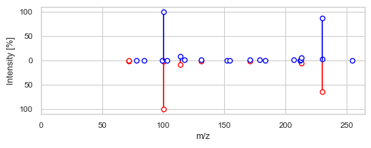
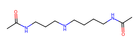
Let’s look at the retrieved library spectra for our query spectra. First, let’s look at the confidently matched spectrum with a high DreaMS similarity.

[17]:

i = df_top1['i'].iloc[25]
df_i = df[df['i'] == i]
for _, row in df_i.iterrows():
    i, j = row['i'], row['j']
    print(f'Library ID: {row["library_ID"]} (top {row["topk"]} hit)')
    print(f'Query precursor m/z: {msdata.get_prec_mzs(i)}, Library precursor m/z: {msdata_lib.get_prec_mzs(j)}')
    print('DreaMS similarity:', row['DreaMS_similarity'])
    print('Modified cosine similarity:', row['Modified_cosine_similarity'])
    su.plot_spectrum(spec=msdata.get_spectra(i), mirror_spec=msdata_lib.get_spectra(j))
    display(Chem.MolFromSmiles(row['library_SMILES']))

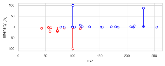
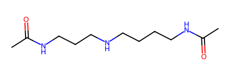
Library ID: MassSpecGymID0236163 (top 1 hit)
Query precursor m/z: 230.18643445964, Library precursor m/z: 230.1863
DreaMS similarity: 0.8856791257858276
Modified cosine similarity: 0.9892408193123613

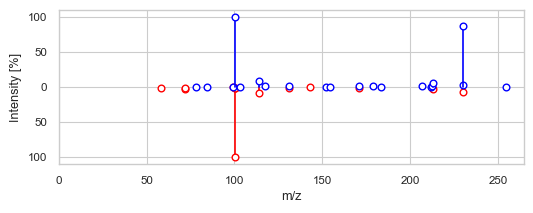
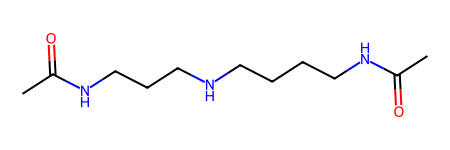
../_images/tutorials_library_matching_19_1.png

../_images/tutorials_library_matching_19_2.png

Library ID: MassSpecGymID0236162 (top 2 hit)
Query precursor m/z: 230.18643445964, Library precursor m/z: 230.1863
DreaMS similarity: 0.8603854179382324
Modified cosine similarity: 0.7990432320842271

../_images/tutorials_library_matching_19_4.png

../_images/tutorials_library_matching_19_5.png

Library ID: MassSpecGymID0236161 (top 3 hit)
Query precursor m/z: 230.18643445964, Library precursor m/z: 230.1863
DreaMS similarity: 0.7787462472915649
Modified cosine similarity: 0.716395852717653

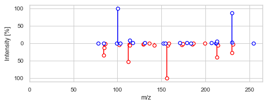
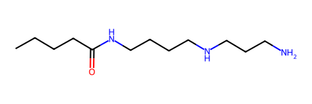
../_images/tutorials_library_matching_19_7.png

../_images/tutorials_library_matching_19_8.png

Library ID: MassSpecGymID0391831 (top 4 hit)
Query precursor m/z: 230.18643445964, Library precursor m/z: 230.223
DreaMS similarity: 0.6461858749389648
Modified cosine similarity: 0.1537209674611311

../_images/tutorials_library_matching_19_10.png

../_images/tutorials_library_matching_19_11.png

Library ID: MassSpecGymID0391832 (top 5 hit)
Query precursor m/z: 230.18643445964, Library precursor m/z: 230.223
DreaMS similarity: 0.6406431198120117
Modified cosine similarity: 0.09253357021617656

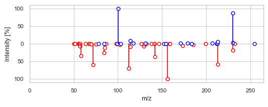
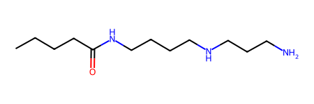
../_images/tutorials_library_matching_19_13.png

../_images/tutorials_library_matching_19_14.png

The top-1 hit demonstrates a strong match, aligning well with the modified cosine similarity. However, annotating a query spectrum with a library spectrum is often impossible due to the limited size of available libraries. In such instances, DreaMS similarity offers an interesting approach, providing insights into the molecular structure even without a definitive match. Let’s examine a case with a less confident hit to illustrate this concept.

[32]:

i = df_top1['i'].iloc[-5]
df_i = df[df['i'] == i]
for _, row in df_i.iterrows():
    i, j = row['i'], row['j']
    print(f'Library ID: {row["library_ID"]} (top {row["topk"]} hit)')
    print(f'Query precursor m/z: {msdata.get_prec_mzs(i)}, Library precursor m/z: {msdata_lib.get_prec_mzs(j)}')
    print('DreaMS similarity:', row['DreaMS_similarity'])
    print('Modified cosine similarity:', row['Modified_cosine_similarity'])
    su.plot_spectrum(spec=msdata.get_spectra(i), mirror_spec=msdata_lib.get_spectra(j))
    display(Chem.MolFromSmiles(row['library_SMILES']))

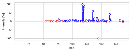
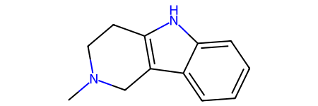
Library ID: MassSpecGymID0240559 (top 1 hit)
Query precursor m/z: 186.980925613972, Library precursor m/z: 187.123
DreaMS similarity: 0.3821600675582886
Modified cosine similarity: 0.005611964348858777

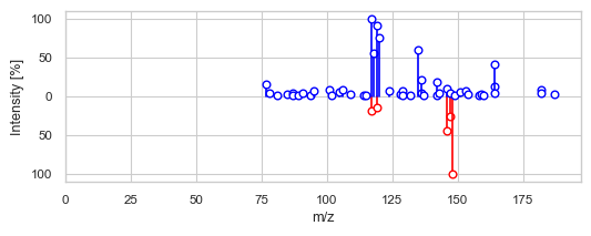
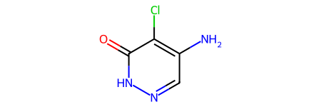
../_images/tutorials_library_matching_21_1.png

../_images/tutorials_library_matching_21_2.png

Library ID: MassSpecGymID0015768 (top 2 hit)
Query precursor m/z: 186.980925613972, Library precursor m/z: 146.0116
DreaMS similarity: 0.3812687397003174
Modified cosine similarity: 0.1472003166482408

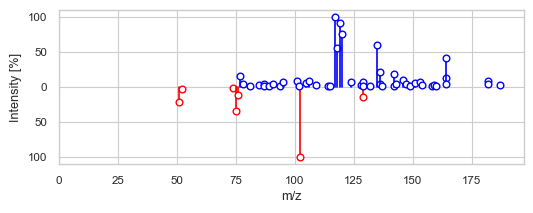
../_images/tutorials_library_matching_21_4.png

../_images/tutorials_library_matching_21_5.png

Library ID: MassSpecGymID0079643 (top 3 hit)
Query precursor m/z: 186.980925613972, Library precursor m/z: 146.0712736972
DreaMS similarity: 0.37886130809783936
Modified cosine similarity: 0.07692617816195739

../_images/tutorials_library_matching_21_7.png

../_images/tutorials_library_matching_21_8.png

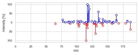
Library ID: MassSpecGymID0117726 (top 4 hit)
Query precursor m/z: 186.980925613972, Library precursor m/z: 187.0865894
DreaMS similarity: 0.3684600591659546
Modified cosine similarity: 0.14840001932798705

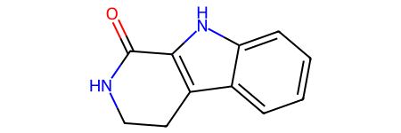
../_images/tutorials_library_matching_21_10.png

../_images/tutorials_library_matching_21_11.png

Library ID: MassSpecGymID0117714 (top 5 hit)
Query precursor m/z: 186.980925613972, Library precursor m/z: 187.0865894
DreaMS similarity: 0.36845511198043823
Modified cosine similarity: 0.1485209819270144

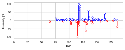
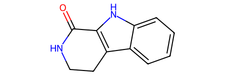
../_images/tutorials_library_matching_21_13.png

../_images/tutorials_library_matching_21_14.png

While the query spectrum cannot be confidently matched to any known library spectrum, the top five hits reveal a consistent pattern: all retrieved molecules, though small in size, contain at least two nitrogen atoms. This observation suggests that the unknown compound represented by the query spectrum is nitrogen-rich. Even without a definitive match, we can still formulate a structural hypothesis for the unknown compound.

Even faster search via approximate nearest neighbors

To achieve even faster library matching, we can use the approach of approximate nearest neighbors (ANN). In this example, we’ll utilize the PyNNDescent library. However, since DreaMS embeddings are 1024-dimensional vectors, they can be seamlessly integrated with any other vector database of your choice for efficient similarity search or other applications (e.g., clustering or visualization).

[33]:

# Build an index for the library
import pynndescent
index = pynndescent.NNDescent(embs_lib, metric='cosine', n_neighbors=50)

[ ]:

# Approximate nearest neighbors search for i-th spectrum (note that the first query may be slow)
neighbors = index.query(embs[[i]])
pd.DataFrame({
    'j': neighbors[0][0],
    'DreaMS_similarity': 1 - neighbors[1][0]  # Convert distances to similarities
})

	j	DreaMS_similarity
0	168540	0.382160
1	62809	0.378861
2	89593	0.368460
3	89581	0.368455
4	117184	0.356404
5	117183	0.355120
6	89605	0.354955
7	41768	0.348629
8	84511	0.347867
9	84520	0.347862

[35]:

# Exact nearest neighbors search for i-th spectrum
df_i[['j', 'DreaMS_similarity']]

[35]:

	j	DreaMS_similarity
19020	168540	0.382160
19021	12627	0.381269
19022	62809	0.378861
19023	89593	0.368460
19024	89581	0.368455

As we can see, the result of the ANN search is very similar to the exact nearest neighbors search (top 1 hit is identical). However, the ANN search is much faster, especially for large libraries.